Terminology​

Introduction​

The OpenID Federation specification was officially published by the OpenID Connect Working Group on May 31, 2024.

The objective of this new specification is to establish a trust relationship between Identity Providers and Relying Parties. As a result, manual provisioning of Relying Parties via a web portal or a dedicated REST API will no longer be necessary.

There are several advantages to using OpenID Federation:

• Reduced human administration.
• Relying Parties can manage their properties, such as the redirect_uri.
• Easily establish trust between Identity Providers and Relying Parties.

This specification is based on concepts from Public Key Infrastructure (PKI), but there are key differences between the two:

• In Public Key Infrastructure, Certificates are used, and the Certificate Authority is installed in the Trusted Root Certificate Authorities certificate store. This store contains the root certificates of all CAs trusted by Windows.

• OpenID Federation uses Entity Statements, represented as JSON Web Tokens (JWT). ach entity involved in the trust chain provides a REST API that exposes operations, as described in section 8 of the specification. Examples include /federation_fetch_endpoint and resolve.

Before proceeding, it is important to understand all the concepts related to Public Key Infrastructure.

Chain of trust in Public Key Infrastructure (PKI)​

The purpose of a Public Key Infrastructure (PKI) is to enable the secure electronic transfer of information for various network activities, such as e-commerce, internet banking, and confidential email.

PKI uses cryptographic public keys linked to a digital certificate, which authenticates the device or user sending the digital communication. Digital certificates are issued by a trusted source, known as a Certificate Authority (CA), and act like digital passports to verify the identity of the sender.

When a client, such as a browser visiting a secure website, receives a digital certificate, it validates whether the issuer of the certificate is in its list of trusted root certificates. If no match is found, the client attempts to resolve the chain of trust by locating the trusted root CA that signed the issuing CA's certificate.

The chain of trust is a crucial concept, as it proves that the certificate originates from a trusted source. Using a certificate store is sufficient to resolve this chain of trust.

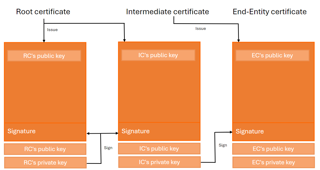
A valid chain of trust consists of three main entities:

• Root CA certificate : A self-signed X.509 certificate that acts as a trust anchor. It is used by all relying parties as the starting point for path validation. The Root CA's private key is used to sign Intermediate CA certificates.

• Intermediate CA certificate : This certificate is positioned between the Root CA and the End-Entity certificate. It is responsible for signing the End-Entity certificates.

• End-Entity certificate : This is the server certificate issued to a website domain.

This chain of trust is also a key concept in the OpenID Federation specification.

Chain of trust in OPENID federation​

The chain of trust in the OpenID Federation consists of more than two Entity Statements.

An Entity Statement is a signed JSON Web Token (JWT). The subject (sub) of the JWT is the entity itself, while the issuer (iss) is the party that issued the Entity Statement. All entities in a federation publish an Entity Statement about themselves, called an Entity Configuration.

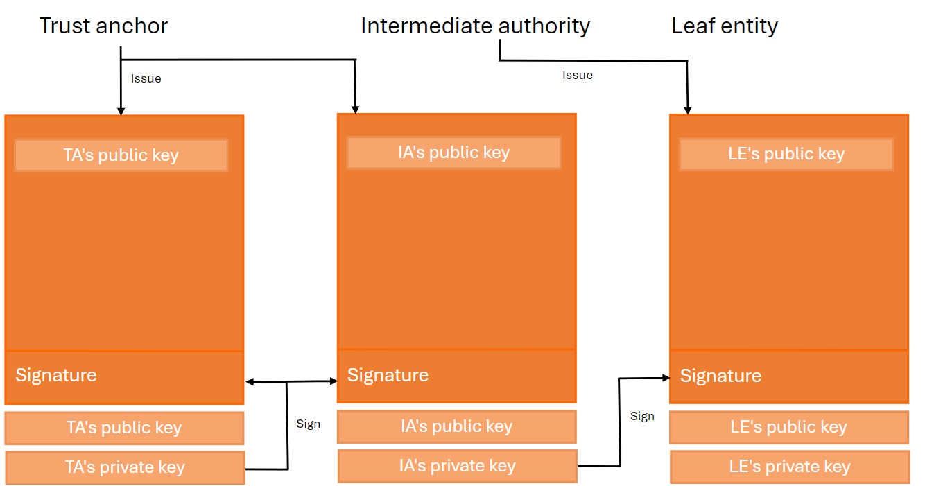
Entities that form the trust chain are categorized as follows:

• Trust anchor : An entity that represents a trusted third party.

• Leaf : In an OpenID Connect identity federation, this refers to a relying party or a protected resource.

• Intermediate : An entity that is neither a leaf nor a trust anchor.

Algorithm to resolve the chain of trust​

The resolution of the trust chain in OpenID Federation is more complex than in Public Key Infrastructure (PKI).

Assume the following architecture is deployed, with trust relationships configured between the following entities:

• Identity Provider and Trust Anchor.

• Relying Party and the Trust Anchor.

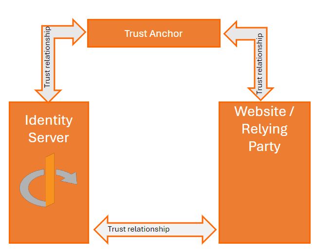
Even if the Relying Party is not registered or configured with the Identity Provider, the Identity Provider can still accept the OPENID Authorization Request from the Relying Party, due to the trust relationship between the two entities.

Suppose the following entities are configured and deployed:

The algorithm used by the Identity Provider to resolve the trust chain consists of the following steps:

1. The Identity Provider receives a request object from the Relying Party.

2. Parse the request object and extract the issuer (iss) (http://localhost:7001).

3. Retrieve the Entity Configuration from the endpoint http://localhost:7001/.well-known/openid-federation.

4. Store the JSON Web Token (JWT) into the trust chain.

5. Parse the JWT and retrieve the list of authority_hints from the payload.

6. For each record in the authority_hints, perform the following actions:

   6.1. Retrieve the Entity Configuration from the authority_hint (http://localhost:7000/.well-known/openid-federation).

   6.2. Parse the JWT and extract the federation_fetch_endpoint.

   6.3. Fetch the Entity Statement of the Relying Party http://localhost:7001 from the Trust Anchor (http://localhost:7000/federation_fetch?sub=http://localhost:7001) and store the result in the trust chain.

7. The final Entity Configuration retrieved from http://localhost:7000/.well-known/openid-federation is the Trust Anchor and must be stored in the trust chain.

8. The Identity Provider checks if the Trust Anchor is trusted and continues processing the request object. The Relying Party will automatically be registered with the Identity Provider.

In the end, the trust chain will contain three records and have the following structure:

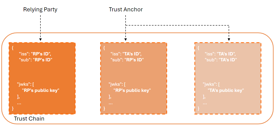
The Relying Party will automatically be registered with the Identity Provider. This process is known in OpenID Federation as the Automatic Registration workflow.

There is another method for Client Registration, which can be found in the chapter on Client Registration.

If the Relying Party is already known to the Identity Provider and the workflow is executed a second time, the Identity Provider will check if the trust chain is still valid. If necessary, the Relying Party's settings will be updated with properties extracted from the openid_relying_party Entity Type.

Federation Policy​

Trust Anchors and Intermediate Entities can define policies that apply to the metadata of their subordinates.

Federations may utilize metadata policies to achieve specific objectives:

• Ensure interoperability between entities : Ensure that the metadata published by OpenID Providers and Relying Parties is interoperable.

• Enforce a security profile: Ensure that the entity metadata complies with a security profile, such as FAPI.

The logic to validate the Federation Policy must be applied after the trust chain has been obtained and validated.

The algorithm to check the Federation Policy consists of the following steps:

1. Ensure the trust chain is valid.

2. Retrieve all Entity Statements from the trust chain and order them from the highest node in the hierarchy (Trust Anchor) to the lowest node (Leaf Entity).

3. For each ordered Entity Statement, fetch the metadata_policy parameter.

   3.1 Retrieve the metadata policy of the previous Entity Statement.

   3.2 Merge the current metadata policy with that of the previous Entity Statement.

   3.3 If the merge is not allowed, produce a policy error.

4. Validate the entity's metadata against the merged metadata policy.

Here is an example of a policy that requires the Relying Party to provide a client_name metadata parameter:

Policy

{
    "metadata_policy": {
        "client_name": {
            "essential": true
        }
    }
}

Difference between PKI and OPENID federation​

The structure of the trust chain in both technologies is similar and consists of comparable components. However, the key difference lies in the terminology and the nature of the entities involved. In PKI, an entity is represented by a certificate, while in OpenID Federation, an entity is represented by an Entity Statement.

X.509 Certificate VS Openid Federation

Entity names

The trust chain algorithm in OpenID Federation is more complex than in PKI. In OpenID Federation, a series of HTTP requests are executed to retrieve a list of Entity Statements, whereas in PKI, the certificate store alone is used.

Relying Party registration​

As discussed in the previous chapter Algorithm to resolve the chain of trust, the OpenID Federation introduces two methods for registering a Relying Party with an Identity Provider: Automatic Registration or Explicit Registration.

Automatic registration​

Automatic registration allows a Relying Party to make authentication requests without a prior registration step with the Identity Provider. Once the authorization request is received by the Identity Provider, it uses the client identifier to resolve the chain of trust and check its validity.

For more information about this type of registration, refer to the documentation. If the chain of trust is valid and the federation policy is satisfied, the client will be automatically registered.

Explicit registration​

In explicit registration, the Relying Party establishes its client registration with the Identity Provider through a dedicated registration request, similar to the Openid Connect Dynamic Client Registration. Instead of submitting its metadata, the Relying Party provides its Entity Configuration or an entire trust chain.

Once explicit registration is complete, the Relying Party can make regular OpenID authentication requests to the Identity Provider.

The expiration time of the client corresponds to the earliest expiration time in the trust chain. When the client expires, the Identity Provider attempts to refresh the trust chain and update the client's metadata accordingly.

Real-World Use Case​

The OpenID Federation standard is used in several real-world scenarios.

OpenID for Verifiable Credential Issuance​

The OpenID Federation is implemented by the OPENID for Verifiable Credential issuance standard.

The API responsible for issuing Verifiable Credentials, such as university diplomas or driver's licenses, uses OpenID Federation to verify whether electronic wallets can be trusted and are authorized to receive the Verifiable Credentials.

The Chain of Trust is passed in the trust_chain parameter. If the chain is valid, the Verifiable Credential is issued and stored in the electronic wallet.

SPID - Public Digital Identity System​

The OpenID Federation standard is also used in Italy within the SPID system (Public Digital Identity System). It allows Italian citizens to select a Digital Identity Provider of their choice to authenticate on any public administration website.

The OpenID Federation provides a trust infrastructure that is:

• Dynamic : Trust can be established dynamically during the first authentication request.
• Scalable : It significantly reduces onboarding costs by following the principle of delegation.
• Transparent : Any entity involved in the federation can build trust autonomously and securely at any time.

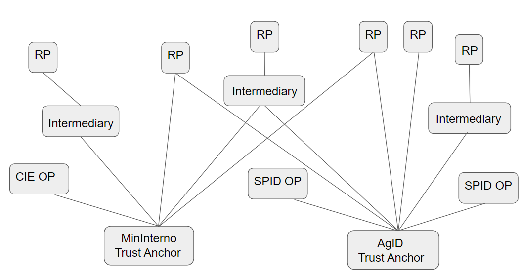
As shown in the diagram above, two trust anchors are configured:

• AgID : A trusted party which within the SPID Federation.

• MinInterno : A trusted party within the Ministry of the Interior.

Any Relying Party with at least one trust relationship with an intermediate entity can fetch all OpenID Provider leaf entities from the Federation Listing endpoint of the trust anchor, extract their metadata, and display the list of Identity Providers.

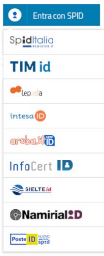
The image below shows the authentication window displayed on a public administration website, where nine Identity Providers are configured:

In the next chapter, we will explain how to implement OpenID Federation with .NET Core.

Demo​

If you want to run a demo of OpenID Federation on your local machine, I recommend following this guide from SimpleIdServer. You'll create a trust chain between a Relying Party and an Identity Server.

Conclusion​

The OpenID Federation standard is highly beneficial for organizations with complex infrastructures, multiple Identity Providers, and numerous Relying Parties. It significantly reduces the time and effort required to manage the configuration of Identity Providers and Relying Parties.

Key advantages include:

• Reduced human administration: No need to use an administration website to create a client in an Identity Provider.
• Self-management by Relying Parties: Relying Parties can manage properties such as redirect_uri.
• Easier trust relationship establishment: Trust between the Identity Provider and the Relying Party can be set up seamlessly.

Overall, developers spend less time configuring authentication in the Relying Party.

Resources​

• https://simpleidserver.com/docs/tutorial/openidfederation#demo, Openid federation

• https://openid.net/specs/openid-federation-1_0.html, OPENID federation 1.0 - draft 36

Introduction​

Like any blogger, every week, I aim to identify popular keywords related to the .NET universe to assist me in crafting my future articles.

To aid me in this task, I am developing a console application in python that retrieves and analyzes articles with the hashtag #dotnet on the dev.to website.

The objective of the article is to comprehend the workings of the Natural Language Processing (NLP) domain through a concrete use case.

The process of keyword extraction comprises the following steps:

1. Retrieval of articles from the dev.to website.
2. Text transformation into vectors.
3. Extraction of keywords.
4. Identification of topics.
5. Data exploration.

Considering that we do not intend to process a large volume of data, performance has not been a determining factor in the choice of algorithms and Python libraries. However, the relevance of the keywords extracted from the articles is of greater importance.

1. Retrieving articles​

After analyzing the HTTP traffic of the dev.to website, I was able to identify a REST API. It exposes an operation that returns the 60 latest articles tagged with #dotnet.

https://dev.to/search/feed_content?per_page=60&page=0&sort_by=published_at&sort_direction=desc&tag_names%5B%5D=dotnet&search_fields=dotnet

Knowing this, we can create a Python script that calls the operation.

import requests

article_result = requests.get("https://dev.to/search/feed_content?per_page=60&page=0&sort_by=published_at&sort_direction=desc&tag_names%5B%5D=dotnet&search_fields=dotnet")

A collection of elements is returned by this operation. Some properties of the element are noteworthy and can be exploited to evaluate the popularity of an article, for example:

• public_reactions_counts : Number of reactions.
• comments_count : Number of comments.

The content of the article is not returned by the HTTP operation. But it is possible to retrieve it using the path property.

import requests
import pandas as pd
import multiprocessing

def read_article(url):
    article_content = requests.get(url['base_url'])
    return { 'article_content': article_content, 'id': url['id'] }

base_url = 'https://dev.to'
result = requests.get(base_url + '/search/feed_content?per_page=60&page=0&sort_by=published_at&sort_direction=desc&tag_names%5B%5D=dotnet&search_fields=dotnet')
json = result.json()
df = pd.json_normalize(json, 'result')
df = df[['id', 'title', 'user_id', 'public_reactions_count', 'comments_count', 'published_at_int', 'reading_time', 'path']]
df.columns = ['Id', 'Title', 'UserId', 'ReactionsCount', 'CommentsCount', 'Published', 'ReadingTime', 'Path']
df.loc[:,'Article'] = [''] * len(df)
links = list(map(lambda p,i: { 'base_url' : base_url + p, 'id' : i }, df['Path'], df.index.values))
    with multiprocessing.Pool() as pool:
        results = pool.map(read_article, links)
    for link in results:
        df.at[link['id'], 'Article'] = link['article_content']

The article is retrieved in its HTML form, but its content is not easily exploitable. This is where the BeautifulSoup library comes into play. It is used to:

1. Clean up the unnecessary.

   1.2. Remove iframe, script tags.

   1.3 Remove code snippets written in different languages.

2. Remove emoticons.

3. Extract the content.

Thus, the read_article function can be rewritten in this way:

def read_article(url):    
    article_result = requests.get(url['base_url'])
    article_soup = BeautifulSoup(article_result.text, features='html.parser')
    [x.extract() for x in article_soup.findAll(True, {"class": ["highlight"]})]
    [x.extract() for x in article_soup.findAll("script")]
    [x.extract() for x in article_soup.findAll("iframe")]
    content = article_soup.find(id='article-body')
    text = content.get_text()
    emoji_pattern = re.compile("["
            u"\U0001F600-\U0001F64F"  # emoticons
            u"\U0001F300-\U0001F5FF"  # symbols & pictographs
            u"\U0001F680-\U0001F6FF"  # transport & map symbols
            u"\U0001F1E0-\U0001F1FF"  # flags (iOS)
    "]+", flags=re.UNICODE)
    article_content = emoji_pattern.sub(r'', text)
    return { 'article_content': article_content, 'id': url['id'] }

The complete code for extracting the content of the articles can be found here.

Now that the articles are ready to be exploited, we can transform the text into vectors.

2. Text to Vector Transformation​

The vectorization process involves converting a string of characters into a vector of numerical values.

There are several transformation algorithms, here are a few: If you would like a complete list of possible algorithms, I invite you to read this article.

In our program, we have chosen the Sentence Transformer as the vectorization process.

Since the emergence in 2017 of the first transformer, introduced by the excellent scientific article Attention is all you need, it has been generally accepted by the NLP community that pre-trained transformers are the most effective means of vectorization and enable the following tasks to be performed efficiently:

• Semantic Textual Similarity (STS) : Comparison of sentence pairs. We may want to identify patterns in datasets, but this is most often used for benchmarking.
• Semantic search : information retrieval (IR) using semantic meaning.
• Clustering : We can cluster our sentences, useful for topic modeling.

The Python program uses the KeyBert library, configured to utilize the all-mpnet-base-v2 model.

Here is the code used to vectorize the articles. The parameter keyphrase_ngram_range is set to (1,2) as we aim to extract keywords consisting of one or two tokens.

file = "articles.csv"
df = pd.read_csv(file)
df["Content"] = df["Title"] + " " + df["Article"]
# 1. Extract embedding
kw_model = KeyBERT(model='all-mpnet-base-v2')
doc_embeddings, word_embeddings = kw_model.extract_embeddings(df["Content"], keyphrase_ngram_range=(1,2))

Now that the articles are transformed into vectors, we can extract the keywords.

3. Keyword Extraction​

There are several Python libraries for extracting keywords.

For a more detailed list of libraries, I invite you to read the article.

The KeyBERT library is the most resource-intensive, but it is more accurate and yields better results because it utilizes the cosine similarity calculation between vectors to choose keywords.

This algorithm has the advantage of considering the context of keyword usage, unlike other algorithms.

Here is the Python code to extract keywords:

content_keywords = kw_model.extract_keywords(df["Content"], doc_embeddings=doc_embeddings, word_embeddings=word_embeddings, keyphrase_ngram_range=(1,2))
keywords = []
for lst in content_keywords:
    keywords.append([component[0] for component in lst])
df["Keywords"] = keywords

Now that the keywords from the articles are extracted, we can group the articles by topic.

4. Topic Identification​

To identify the topics, it is necessary to reduce the dimensionality of doc_embeddings to 2. For this purpose, the UMAP library is used.

# 3. Reduce the doc embeddings
reduced_embeddings = umap.UMAP(n_components=2, n_neighbors=5, min_dist=0.02).fit_transform(doc_embeddings)

You can find more details about the parameters (n_components, n_neighbors, min_dist) on the official website.

Next, the clustering algorithm HDBSCAN is used to identify the topics of the articles.

# 4. Cluster the articles
clusterer = hdbscan.HDBSCAN(min_cluster_size=3)
labels = clusterer.fit_predict(reduced_embeddings)
df["Label"] = [str(label) for label in labels]

Now that we have all the information, we can analyze the data to identify the most popular keywords.

5. Data exploration.​

The 60 latest articles were retrieved on March 27, 2024.

To retrieve the most popular keywords, which were sorted in descending order based on the ReactionsCount column, the following Python script was executed:

# 5. Get trending keywords
sorted_df = df.sort_values(by=['ReactionsCount'], ascending=False)
print(sorted[["ReactionsCount", "Label", "Keywords"]][:30])

As a result, the most popular keywords are:

• azure openai
• primary constructors
• loop execution
• iterate
• coding assistant

By grouping the articles by topic and calculating the sum of reactions, we observe that the topic which received the most reactions is the one discussing challenges in .NET.

# 6. Get topics with the most reactions
grp = df.groupby(by=["Label"])
count = grp.size().to_frame(name='counts')
res = count.join(grp.agg({'ReactionsCount':'sum'}).rename(columns={'ReactionsCount': 'TotalReactions'}))
print(res.sort_values(by=['TotalReactions'], ascending=False))

Conclusion​

The source code of the Python application can be found here.

The results obtained by the application are satisfactory and accurate. They enable the rapid identification of the most popular keywords from the latest 60 articles.

This application is not easily usable by a blogger and requires some improvements, which will be the subject of future articles.

Resources​

Introduction​

In this article, we will cover various theoretical topics with the aim of implementing a neural network in C# that is capable of recognizing a digit present in an image.

The article is divided into three parts:

1. Presenting the key principles of a neural network.
2. Explaining the architecture of a Convolutional Neural Network.
3. C# source code.

If you are familiar with the concept of neural networks, feel free to skip this chapter and proceed to the next.

Neural Network Architecture​

A neural network is composed of multiple interconnected layers, with neurons forming connections between them.

There are three types of layers.

1. Input Layer​

The input layer consists of neurons representing the features of the input data. Each neuron corresponds to a feature, and its value represents the value of that feature.

2. Hidden Layer​

Between the input layer and the output layer, there can be multiple hidden layers.

Generally, each neuron in a hidden layer is connected to all neurons in the preceding layer, a configuration known as a fully connected or dense layer type.

A hidden layer has two parameters:

• weights : Each connection between two neurons has a weight, which is a parameter that influences the amount of information transmitted between them.

• bias : Constant assigned to a layer.

These two parameters are part of the calculation formula for the WeightedSum :

These two parameters are adjusted during the learning process, specifically during the back propagation step.

An activation function can then be applied to the calculated parameter $SumWeighted$. Generally, the same type of function is chosen for all hidden layers. The choice depends on the nature of the neural network; for example, a CNN or MLP network typically uses ReLU.

There are several types of functions, listed as follows.

3. Output Layer​

The final layer of the neural network is the output layer. It shares the same structure as a hidden layer as it comprises multiple neurons and may have the parameters weights and bias.

This layer receives information from the last hidden layer and conducts computations to predict or classify the received data.

Depending on the nature of the problem the neural network aims to solve, you can select one of these layers:

Neural network training algorithm​

Now that you have an overview of the components that constitute a neural network.

We will explain the various steps to train a neural network, outlined as follows:

1. Initialize the parameters of all layers : weights ou bias.

2. Execute the following steps N times.

   2.1 For each layer, execute the forward propagation step.

   2.2 Calculate the error.

   2.3 For each layer, execute the backward propagation step.

1. Initialize the parameters​

The learning parameters of the layers, such as weights and bias, must be initialized with random values.

According to the Xavier Initialization method, this step is more crucial than one might think because if the initial values are too large or too small, then the training of the neural network becomes inefficient.

Depending on the nature of the layer, it may not be necessary to initialize these parameters.

2. Forward propagation​

The Forward propagation step is executed when a layer receives data from another. It consists of the following steps:

1. For each neuron, calculate the sum weighted : $sm = \sum_{i=1}^{n}xi *wi$.

   1.1. $wi$ is the value of the weight that the neuron has with the i-th neuron.

   1.2. $xi$ is the value of the i-th neuron.

2. Add the sum-weighted to the bias parameter : $t = b + \sum_{i=1}^{n}xi *wi$.

3. Call the activation function: $f(b + \sum_{i=1}^{n}xi *wi)$.

3. Calculate the error.​

When data is received from the last layer, the result can be compared with the expected outcome. The difference indicates the error that the network made during its prediction.

There are various methods to calculate the error; once again, the choice depends on the nature of the problem.

4. Backpropagation​

The error calculated by the loss function is then propagated through the various layers.

The learning process begins with Backpropagation aiming to reduce the cost of the loss function by adjusting the parameters weights and bias of the different layers.

The degree of adjustment of the variables weights and bias is calculated by gradients. They help understand how a variable like the weight can influence the total result Loss.

Convolutional Neural Network (CNN)​

The neural network tailored for image recognition is of the Convolutional type.

The typical architecture of a CNN consists of four layers."

• Input layer : Extract the data from an image in one of the two formats:

  • Three two-dimensional RGB matrices.

  • A two-dimensional matrix with grayscale values.

• First hidden layer : Convolutional layer.

• Second hidden layer : Max pooling layer.

• Output layer : softmax layer.

1. Convolutional Layer​

Before describing the structure of this layer, it is important to understand the concept of a convolution matrix.

A convolution matrix, also known as a kernel, is a two-dimensional matrix. When applied to an image, it enables various effects, as demonstrated in the example below. For a comprehensive list of filters, please refer to the Wikipedia website.

Operation	Kernel	Result
Edge detection

Assuming the image has been extracted into a grayscale matrix of size $(imw * imh)$, the convolution algorithm consists of the following steps:

1. Create a convolution matrix/kernel of size $(kw * kh)$. By default, the matrix will have a size of 3x3.

2. Create an output matrix of size $(imw - kw + 1) * (imh - kh + 1)$.

3. Retrieve all windows from the input image. The center of the kernel matrix is used as a pointer, and the algorithm moves the pointer over each column and each row of the image. The area covered by the kernel, also called a window, is then stored in a list called windows.

4. For each element in the windows list:

   4.1. Multiply the value by the kernel.

   4.2. Calculate the average and store the result in the output matrix.

To summarize, here is the mathematical equation to calculate each element of the output matrix.

• $kernel(kx;ky)$ : the coefficient of the convolution kernel at position kx,ky.
• $img(mx,my)$ : the data of the pixel that corresponds to img(mx,my).
• $F$ : Sum of the coefficients of the kernel.

By applying this algorithm multiple times, there is a risk of losing pixels on the edges of the image. To address this issue, the padding parameter has been introduced.

Padding parameter​

This parameter indicates the number of pixels to be added to the edges of the image.

Assuming that the padding parameter is defined by the variable p, the size of the output matrix will be calculated as follows:

In many cases, the padding value is set to $(kw-1,kh-1)$ so that the output image has the same size as the input image.

Stride parameter​

For each pixel of the image, a convolution window is applied. This operation can be resource-intensive, especially when the algorithm is applied to a large image.

To decrease the number of iterations, the stride parameter has been introduced. It defines the number of elements to be skipped in the width and height of the image. By default, this parameter is set to (1,1).

Assuming that the stride parameter is defined by the variable s, the size of the output matrix will be calculated as follows:

Forward propagation​

A convolutional layer consists of 1 or more neurons, and each neuron has its own convolution window.

During the forward propagation phase, each neuron executes the convolution algorithm on a window of the image.

Here are the main steps of the forward propagation algorithm:

1. Retrieve all windows of the input image.

2. For each input window, execute the convolution algorithm of each neuron and store the result in a list.

3. Store the list in the output matrix.

Here is the architecture of a neuron in a convolutional layer.

Backward propagation​

Given that in the article, the convolutional layer does not have bias parameters and activation functions, the backward propagation algorithm amounts to computing this formula :

2. Max Pooling layer​

This layer consists of no neurons and does not have any bias or weights parameters. It reduces the size of the input matrix by applying the max operation to each window of the input matrix.

Its objective is twofold:

1. Reduce dimensionality.
2. For each region, find the maximum.

Forward propagation​

The forward propagation algorithm consists of the following steps:

1. Define the size of the pooling window $(pw * ph)$.

2. Create an output matrix of size $(iw / pw) * (ih / ph)$.

3. Divide the input matrix into several windows of size $(pw * ph)$.

4. For each window of the matrix, find the maximum value and assign this value to the cell of the output matrix.

Backward propagation​

Given that the Pooling layer has no learning parameters, weights, or bias.

The backward propagation algorithm simply reconstructs a matrix of the same size as the last matrix received by the layer. Here are the main steps of the algorithm:

1. Create an output matrix of the same size as the input matrix.

2. Divide the matrix into several windows of size $(pw * ph)$.

3. For each cell of each window, if the element is not the maximum, set it to 0; otherwise, take the gradient of the error.

3. Softmax layer​

The activation dense layer softmax consists of one or more neurons and has the learning parameters weights and bias. The number of neurons is equal to the number of classes to predict.

The softmax function is used to calculate the probabilities of belonging to each class.

Here is the architecture of a softmax neuron.

Forward propagation​

The forward propagation algorithm consists of the following steps:

1. Define the number of classes in a variable n.

2. For each class, create a neuron and initialize its weight parameter.

3. Initialize the layer's bias parameter.

4. For each neuron, multiply the input matrix by its weight and store the result in a variable $Weights = \sum_{i=1}^{n}xi *weighti$.

5. Calculate the sum with the bias and store the result in a variable $SumWeighted = bias + Weights$.

6. Finally, execute the activation function on each class $softmax(ci) = \frac{exp(ci)}{\sum_{i}^{n}exp(i)}$.

Backward propagation​

The softmax layer has two learning parameters that need to be updated, and a variable learningRate which weighs the importance of the partial derivatives to update these parameters.

The algorithm must be able to compute the partial derivatives for these two parameters.

The derivative $\frac{\delta Loss}{\delta out}$ is quite simple to calculate.

If the predicted class is different from the expected one:

If the predicted class is the same as the expected one:

The derivative $\frac{\delta net}{\delta weight}$ is equals to :

The derivative $\frac{\delta out}{\delta bias}$ is equals to 1.

The last derivative, $\frac{\delta out}{\delta net}$, is more complex to calculate. If you desire a complete demonstration, I invite you to read the article published on medium.

Once all these partial derivatives are calculated, the parameters can be updated as follows:

C# implementation​

The source code of the C# project can be found here.

The project uses a MINST dataset from the kaggle website to train the Convolutional Neural Network.

After 3 iterations performed on a dataset of 5000 entries, the achieved performance is quite satisfactory.

The accuracy is approximately 85%!

Conclusion​

Congratulations! You've reached the end of this article. 😉

The C# implementation is not optimal and can still be improved.

For production use, I recommend using the excellent library keras.

Resources​

• https://observablehq.com/@lemonnish/cross-correlation-of-2-matrices, Cross-correlation of 2 matrices

• https://www.ibm.com/topics/convolutional-neural-networks, What are convolutional neural networks?

• https://developer.nvidia.com/discover/convolution#:~:text=The%20convolution%20algorithm%20is%20often,convolution%20operation%20is%20called%20deconvolution., Convolution

• https://web.pdx.edu/~jduh/courses/Archive/geog481w07/Students/Ludwig_ImageConvolution.pdf, Image Convolution

• https://d2l.ai/chapter_convolutional-neural-networks/conv-layer.html#fig-correlation, Convolutions for image

• https://towardsdatascience.com/a-comprehensive-guide-to-convolutional-neural-networks-the-eli5-way-3bd2b1164a53, A Comprehensive Guide to Convolutional Neural Networks — the ELI5 way

• https://victorzhou.com/blog/softmax/, Softmax

• https://www.sciencedirect.com/topics/computer-science/convolutional-layer, Convolutional Layer

• https://medium.com/@nerdjock/deep-learning-course-lesson-5-forward-and-backward-propagation-ec8e4e6a8b92, Forward and Backward Propagation

Introduction​

The naive implementation of the SGD algorithm presented in the first part is not efficient and can be improved by addressing several points.

• The paper Parallelized Stochastic Gradient Descent suggests executing the algorithm on multiple machines in parallel.

• Utilizing the GPU for matrix computations.

Supporting Parallelism​

The main idea is to divide the dataset into subsets/mini-batches and distribute them across multiple machines (learners/processing units).

This method was initially proposed by Google's DistBelief. It uses a central parameter server (PS) that updates the learning model with gradients calculated by the learning nodes.

There are two modes for updating the learning model:

1. Synchrone : The parameter server waits to receive gradients from all learning nodes before updating the model parameters. This approach takes longer and is riskier, as it requires the completion of execution of a portion or all of the nodes.

2. Asynchrone : The parameter server does not wait for the learning nodes. There is a risk that learning nodes execute the algorithm on an outdated version of the model.

The synchronous configuration consists of three methods:

Full Sync SGD : The parameter server (PS) waits to receive the gradient calculation from all learning nodes.

K-Sync SGD : The parameter server (PS) waits to receive K gradient calculation results, where each result comes from a different node. When received, all ongoing calculations on the nodes are canceled. Here, for each iteration, a mini-batch is distributed to each learning node.

K-batch-sync SGD : The parameter server (PS) waits to receive K gradient calculation results, where one or more results can come from the same node.

The asynchronous configuration consists of three methods:

Async SGD : As soon as the parameter server (PS) receives the gradient calculation from a learning node, it updates the learning model.

K-async SGD : The parameter server (PS) waits to receive K gradient calculation results, where each result comes from a different node. Here, for each iteration, a mini-batch is distributed to each learning node.

K-batch async SGD : The parameter server (PS) waits to receive K gradient calculation results, where one or more results can come from the same node.

Unlinke the synchronous mode, the asynchronous mode accepts all results from learning nodes and does not cancel ongoing executions.

At each iteration, if more than one gradient has been received by the PS server, we calculate the average and use this value to update the learning model parameters. Here is the formula for updating the parameter:

• $l$ : denotes the index of the K learners that contribute to the update at the corresponding iteration.
• $\tau_{l,j}$: is one mini-batch of m samples used by the l-th learner at the j-th iteration.
• $\xi_{l,j}$: denotes the iteration index when the l-th learner last read from the central PS.
• $g(w_{\tau(l,j)},\xi_{l,j}) = \frac{1}{n} * \sum_{}^{} \nabla f(w_{\tau(l,j)},\varepsilon_{l,j})$ : average gradient of the loss function evaluated over the mini-batch $\tau_{l,j}$.

Here is the K-batch async SGD algorithm.

Algorithm for the PS server to update the parameters w and itp of a complex-shaped linear function.

1. Define the number of learning nodes N.

2. Define the number of mini-batch K required to update the model parameters.

3. Define the number of iterations epoch.

4. Define the learning rate η. This determines the step size at each iteration while moving toward a minimum of a loss function.

5. Initialize the vector w for weight.

6. Initialize the variable itp for intercept.

7. for i = 1 .... epoch

   7.1 for n .... N do in parallel

   7.1.1 Randomly shuffle samples in the training set and store the result in the tx and ty variables.

   7.1.2 Send the variables tx, ty, w and itp to node k

   7.2 Wait to receive K mini-batches and store the results in two variables nwi and nitpi .

   7.3 $w_{j+1} = w_{j} - \frac{\eta}{K} \sum_{l=1}^{K} (nwi)$

   7.4 $itp = itp - \eta * \sum_{\eta}^{K}(nitpi)$

Algorithm for a learning node to calculate the gradient of a complex-shaped linear function.

1. Receive the mini-batch tx and ty.
2. Receive the parameter w.
3. Receive the parameter itp.
4. Calculate the number of observations N.
5. Calculate the gradient $g = \frac{1}{N} \sum_{i}^{N} -2 * wT * tx * (ty - (itp + w*tx))$
6. Calculate the intercept $itp = \frac{1}{N} * \sum_{i}^{N} -2 * itp * (ty - (itp + w*tx))$
7. Send the variables g and itp to the PS server.

GPU​

As you may have noticed in the previous chapter, both the parameter server and learning nodes perform computations on matrices.

It is recommended to carry out such calculations on the GPU, especially when dealing with large matrices.

If you are not familiar with the key concepts of a GPU, I encourage you to read the next chapter; otherwise, proceed to the CUDA chapter.

CUDA​

In this article, we use CUDA C++, an extension of C++ that enables developers to define kernels, which, when invoked, are executed N times in parallel by N different CUDA threads.

The thread identifier is calculated as follows: idx = threadIdx.x + blockIdx.x * blockDim.x. The parameters for this formula are as follows:

• BlockDim : Dimension of a block, corresponding to the number of threads.
• BlockIdx : Index of the block in a grid.
• ThreadIdx : Index of the thread in a block.

CUDA introduces the following entities:

• Thread : An abstract entity representing the execution of the kernel.
• Block : Composed of multiple wraps, and each wrap has 32 threads.
• Grid : Blocks are combined to form a grid.

During their execution, CUDA threads have access to different memory spaces, including but not limited to:

• Register : Each thread has its own private memory.
• Shared memory : Each Block has memory shared among all its threads. This memory has the same lifespan as the block.
• Global GPU memory : All threads have access to global memory.

If you want more information on the subject, I recommend reading the excellent programming guide https://docs.nvidia.com/cuda/cuda-c-programming-guide/index.html#programming-model.

Now that you have an overview of all the involved entities when developing with CUDA, you can write the algorithm for calculating the gradient of a function on the GPU, considering the following points:

• If the matrix is too large, it can be divided into several tiles. The CUDA documentation explains how this works.
• Reduce the number of interactions between a thread and the Global GPU Memory; the thread should, whenever possible, use shared memory.

You are now ready to write your first matrix calculation algorithm on a GPU.

Performing Matrix Operations​

The matrix operation most commonly used in the SGD algorithm is the multiplication of a matrix with a vector.

This article on GPU matrix-vector product (gemv) explains clearly the various ways to implement this algorithm.

In our case, we will not implement the algorithm from scratch or others. Instead, we will use the BLAS library provided by CUDA, which is optimized for performing this type of calculation.

It offers several useful functions for writing an optimized version of the SGD algorithm:

We used the ILGPU library to write our algorithm; you can find the source code here https://github.com/simpleidserver/DiveIt/Projects/SGDOptimization/GPUMathUtils.cs.

Performance​

We conducted several tests to compare performance.

All tests were run on the same dataset.

Sequential SGD - CPU (6837 MS)

Sequential SGD - GPU (3243 MS)

Parallel SGD - CPU (4602 MS)

Parallel SGD - GPU (2911 MS)

As you can see, the performance is much better when the GPU is used to compute matrices. Even though the project does not distribute the computational load of the function gradient across multiple nodes but across multiple threads, the performance remains entirely acceptable.

Conclusion​

The proposed algorithm is not ready for use in a .NET library for production. However, understanding it can help you choose a library for machine learning.

To choose a library, you should check if it supports the following points. They are crucial as they will help reduce the training time of an ML model.

• Capable of supporting parallelism.
• Capable of supporting execution on one or multiple GPUs.

The source code of the project can be found here https://github.com/simpleidserver/DiveIt/tree/main/Projects/SGDOptimization.

Ressources​

Introduction​

In this article, we will implement the Stochastic Gradient Descent Regression algorithm from scratch in C#. This algorithm is well-known and widely used in the field of Machine Learning. It will be utilized for performing Linear Regression on both simple and complex forms.

If you are not familiar with the concept of a Regression function, please read the following chapter. Otherwise, feel free to skip directly to the Gradient Descent chapter.

Regression Versus Classification problems​

Variables of a function can be characterized as either quantitative or qualitative (also known as categorical). Quantitative variables take on numerical values. Examples include a person's age, height, or income. In contrast, qualitative variables take on values in one of K different classes, or categories. Examples of qualitative variables include a person's gender (male or female), the brand of product purchased (branch A, B or C).

We tend to refer to problems with a quantitative response as regression problem, while those involving a qualitative response are often referred to as classification problems.

Least squares linear regression is used with a quantitative response, whereas Logistic regression is used with a qualitative (two-class, or binary) response.

Gradient Descent​

A Gradient Descent function is an iterative algorithm designed to find the minimum of a loss function. This algorithm can be applied to any differentiable function.

Here are the steps of the algorithm:

1. Initialize the vector `w` for all parameters. These parameters are computed by the algorithm.
2. Define the number of iterations `epoch`.
3. Define the learning rate `η`. It determines the step size at each iteration while moving toward a minimum of a loss function.
4. for i = 1 .... epoch do

   4.1 $w = w - η ∇ Qi(w)$

We have chosen to apply this algorithm to both Simple and Complex forms of Linear expressions.

Gradient Descent on Simple Linear Expression​

A simple linear function has this form.

The best loss function to choose for evaluating the performance of the Gradient model is the Mean Squared Error (MSE).

f(xi) is the prediction that the function f provides for the ith observation.

To calculate the gradient of the $MSE$ / $Qi(itp,w)$ function, it is necessary to determine the partial derivatives with respect to the parameters $\frac{\delta}{\delta itp}$ and $\frac{\delta}{\delta w}$ . The chain rule is used to compute them.

For the function f(g(x)), its derivative is f'(g(x)) * g'(x).

Here are the details of the partial derivatives calculations:

Here is the updated gradient algorithm to minimize the loss function of a simple linear function.

1. Initialize the vector x with values.

2. Initialize the vector y with values.

3. Initialize the variable w for weight.

4. Initialize the variable ipt for intercept.

5. Assign random values to these two variables.

6. Define the number of iterations epoch.

7. Define the learning rate η.

8. for i = 1 .... epoch do

   8.1 $w = w - \eta * (\frac{1}{N} \sum_{i}^{n} -2 * xi * (yi - (itp + w * xi)))$

   8.2 $itp = itp - \eta * (\frac{1}{N} \sum_{i}^{n} -2 * (yi - (itp + w * xi)))$

A simple-shaped function may not be sufficient for you, as you have more than 2 parameters to calculate.

In this situation, you need to use the Gradient Descent algorithm to calculate all the parameters of your complex linear function.

Gradient Decent on complex linear expression​

A complex linear function has this form:

Here, the values of the variables xi can be represented in the form of a matrix of size (O, V), where O represents the number of observations, and V represents the number of variables. The variable w can be represented as a vector of size V.

The algorithm is very similar to that applied for a simple linear function but contains a few differences.

1. Initialize the vector x with values.

2. Initialize the vector y with values.

3. Initialize the variable w for weight.

4. Initialize the variable ipt for intercept.

5. Assign random values to these two variables.

6. Define the number of iterations epoch.

7. Define the learning rate η.

8. for i = 1 .... epoch do

   8.1 $w = w - \eta * ( \frac{1}{N} * \sum_{i}^{n} -2 * wT * xi * (yi - (itp + w * xi)))$

   8.2 $itp = itp - \eta * ( \frac{1}{N} * \sum_{i}^{n} 2 * itp * (yi - (itp + w*xi)))$

At step 8.1, the matrix w must be transposed. For more information on this operation, refer to this site https://en.wikipedia.org/wiki/Transpose.

At first glance, this algorithm works well on small-sized matrices but is not suitable for large matrices due to a risk of memory loss. To address this issue, the Stochastic Gradient Descent algorithm has been introduced.

Stochastic Gradient Descent​

The idea of the algorithm is to take a random dataset from the variables x and y and apply the Gradient Descent algorithm to it. This algorithm diverges slightly from the previous one:

1. Initialize the vector x with values.

2. Initialize the vector y with values.

3. Initialize the variable w for weight.

4. Initialize the variable ipt for intercept.

5. Assign random values to these two variables.

6. Define the number of iterations epoch.

7. Define the learning rate η.

8. for i = 1 .... epoch do

   8.1 Randomly shuffle samples in the training set and store the result in the tx and ty variables.

   8.1 $w = w - \eta * ( \frac{1}{N} * \sum_{i}^{n} -2 * wT * txi * (tyi - (itp + w * txi)))$

   8.2 $itp = itp - \eta * ( \frac{1}{N} * \sum_{i}^{n} 2 * itp * (tyi - (itp + w*txi)))$

Now that you have an overview of the Gradient Descent algorithm, we will develop a naive implementation in C# of the Stochastic Gradient Descent algorithm.

C# implementation​

To be able to write the Stochastic Gradient Descent algorithm, we use two classes, CPUMathUtils and MathUtils. These classes facilitate matrix and vector operations, and you can find their source code on GitHub : https://github.com/simpleidserver/DiveIt/Projects/SGD.

Create a class GradientDescentRegression with a static function Compute.

public static void Compute(
    double learningRate,
    int epoch,
    double[,] x,
    double[] y,
    bool isStochastic = false,
    int batchSize = 0)

Initialize the variables, such as intercept and an empty vector for w.

int nbSamples = x.GetLength(0);
var nbWeight = x.GetLength(1);
var w = MathUtils.InitializeVector(nbWeight);
double itp = 0;
var lst = new List<double>();

Create a loop where the number of iterations is equal to epoch.

for (var step = 0; step < epoch; step++)
{

}

In this loop, add the logic to randomly draw a dataset of size batchSize if isStochastic is true.

var tmpX = x;
var tmpY = y;
if(isStochastic)
{
    var shuffle = MathUtils.Shuffle(x, y, nbSamples, nbWeight, batchSize);
    tmpX = shuffle.a;
    tmpY = shuffle.b;
}

Calculate the new value of y (itp + w*txi)

var newY = CPUMathUtils.Add(
  CPUMathUtils.Multiply(tmpX, w),
  itp);          

Calculate the lose factor (losefactor = tyi - (itp + w*txi))

var loseFactor = CPUMathUtils.Substract(tmpY, newY);

Update the w vector (w = w - η * (1/N Σ(i/n) -2 * wT*txi * (loseFactor)))

var tmp = CPUMathUtils.Multiply(
    CPUMathUtils.Divide(
        CPUMathUtils.Multiply(
            CPUMathUtils.Multiply(
                CPUMathUtils.Transpose(tmpX),
                loseFactor
            ),
            -2
        ),
        nbSamples
    ),
    learningRate);
// 4. Update weight
w = CPUMathUtils.Substract(w, tmp);

Update the intercept (itp = itp - η * (1/N Σ(i/n) 2 * itp * (loseFactor)))

itp -= learningRate * (CPUMathUtils.Multiply(loseFactor, -2).Sum() / nbSamples);

Conclusion​

Congratulations! 🥳

If you have reached the end of the article, it may mean that you have successfully implemented the Stochastic Gradient Descent algorithm for a complex linear function. This algorithm is not intended for use in a library as it is not optimized and cannot work on non-convex functions. Therefore, I suggest using a library such as sklearn for linear regression.

In future articles, we will explain how to improve the performance of the algorithm.

Source code​

You will find the source code at this link: https://github.com/simpleidserver/DiveIt/tree/main/Projects/SGD.

Resources​

Introduction​

The goal of this tutorial is to give you an overview of the Dotnet Runtime project. It is intended for developers at all experience levels.

We will explain the various steps that enable the transformation of C# code into native code, executable on any type of machine architecture, such as OSX, Unix-x64, etc.

The transformation process is constructed as follows:

This process can be broken down into two distinct parts :

• The first part involves compiling the C# code into intermediate code.
• The second part involves compiling this intermediate code into native code on-the-fly during program execution.

We will explain each part in the following chapters.

Compile the C# code into intermediate code​

Imagine you have the following C# file. The initial step is to convert the C# code into intermediate code. To achieve this, you must execute the dotnet build command.

Console.WriteLine("Hello world!");
Console.ReadLine();

This command is a part of the dotnet SDK project: https://github.com/dotnet/sdk, and it performs the following actions:

1. Resolves the path of the MSBuild.dll file, which must be present in the root directory of your DOTNET SDK.
2. Executes the command MSBuild <projectName> -t:Rebuild -consoleloggerparameters:Summary.
3. The MSBUILD project, whose source code is located at this address https://github.com/dotnet/msbuild, uses the Roslyn library to compile the C# code into intermediate code (IL).

The compilation process consists of several steps:

1. Tokenizer : In the context of a compiler, tokenization (also known as lexing or lexical analysis) is the process of converting the source code into a sequence of strings with assigned meanings (tokens). The program that performs tokenization is called a tokenizer or lexer.
2. Parser : In the parsing phase, output from the tokenization phase is used to build a data structure named an abstract syntax tree, giving a structural representation of the input while checking for correct syntax.
3. Declaration : Source and imported metadata are analyzed to form named symbols.
4. Binding : Match identifiers in the code to symbols.
5. IL Emission : Intermediate Language is emitted with all the information.

Now that the intermediate code has been generated, we can proceed with the program's execution.

Compilation of the intermediate code on-the-fly​

Execute the command dotnet run to launch the execution of your application.

Virtual Machine​

Upon its launch, the Virtual Machine must first be initialized, and it performs a sequence of actions:

1. Set up the infrastructure that needs to be in place before anything else can run.
2. Initialize the core, low-level components.
3. Start up the low-level components, i.e., error handling, profiling API, debugging.
4. Start the main components, i.e., Garbage Collector (GC), AppDomains, Security.
5. Finalize the setup and then notify other components that the Virtual Machine has started.

Once the Virtual Machine is initialized, it passes the intermediate code to the Just-In-Time compiler. There are two contracts between the Just-In-Time compiler and the virtual machine, allowing for bilateral communication between these two components

The ICorJitCompiler interface (https://github.com/dotnet/runtime/blob/4765dd1b9f1aa58f16d6922438bcc6cb01b4a666/src/coreclr/inc/corjit.h) serves as the entry point for the Virtual Machine and includes several important methods, such as:

• compileMethod: The Virtual Machine passes an object ICorJitInfo that holds the IL code.

The ICorJitInfo interface (https://github.com/dotnet/runtime/blob/b8e1296c832858e7f4b0eb2949afa73147a91981/src/coreclr/inc/corinfo.h) is an interface implemented by the Virtual Machine. It comprises a large number of methods and is used by the Just-In-Time compiler to look up metadata tokens, traverse type signatures, compute field and vtable offsets, and find method entry points.

In our case, the compileMethod method is crucial as it contains the logic to compile the intermediate code into native code.

Just-In-Time compiler​

Here are the most important steps:

1. Importation : For each Statement instruction, we will create the HIR form. The HIR form of int Foo(int x) => x * 2 is:

STMT 0
*         RETURN          INT
\--*      MUL             INT
   +--*   LCL_VAR         INT  arg0
   \--*   CNS_INT         INT  2

2. Clean and optimize

   2.1 Morphing : Including a certain number of transformations, for example, to improve performance. The operation x * 2 can be replaced by a left bit shift operation. The HIR form then becomes :

   STMT 0
   *         RETURN          INT
   \--*      LSH             INT
      +--*   LCL_VAR         INT  arg0
      \--*   CNS_INT         INT  1
   

   2.2 Inlining : Determines whether a function call is likely to be a good candidate for inlining by estimating the size of the native code of the function. If the situation is advantageous, a Compiler object is created, and the nodes are copied into this object after the importation phase has been executed.

   2.3 Optimize layout : The goal here is to eliminate redundant Basic Blocks that will never be executed. For instance, in the following code, the instruction block throw new Exception("Sid"); is disregarded because the condition is never fulfilled.

   if ('B' == 'C')
       throw new Exception("Sid");
   

   2.4 Building SSA form : The goal here is to remove unnecessary variables.

3. Rationalization : Eliminating the parental context in trees results in a transition from a hierarchical model (HIR) to a linear model (LIR).

4. Emitter : For each block, we generate the function prologue, body, and epilogue, and then emit the result into memory. The code is located in the emitarm.cpp class (https://github.com/dotnet/runtime/blob/b8e1296c832858e7f4b0eb2949afa73147a91981/src/coreclr/jit/emitarm.cpp).

Now that the native code has been emitted, the compileMethod function returns a pointer to it, which can then be executed by the virtual machine.

Conclusion​

Now that you have a comprehensive understanding of the various components involved in just-in-time compilation, we will describe in the upcoming articles different sections of the DOTNET RUNTIME library that seem interesting to me. Feel free to leave a comment if you have any remarks 😀

Resources​